In this blog we will explore the concept of volatility decay on leveraged assets.

What is volatility decay?

Volatility decay is an observation made on leveraged assets, more specifically how their compounded-returns compare to those of the non-leveraged versions. The phenomena arises when a sequence of leveraged movements compound to a value that is different than the leverage multiple of non-leveraged movements, which disproves the perception that investing in leveraged assets will give you exactly leveraged returns.

At the core is the fact that the relationship between compounding of returns and compounding of linear multiples of those returns, is not linear.

Volatility decay over a period for a leveraged asset can be formalised as:

Volatility Decay = leverage * unleveraged returns - leveraged returns

For example, if no-leverage movements are 5% then -10% respectively, the net return is -5.5% (1.05 * 0.90 = 0.945).

For a 2x leveraged asset, the movements then are 10% and -20%, with net return being -12%. So volatility decay after 2 movements is 2*(-5.5%) - (-12%) = 1%, meaning someone holding a long 2x leveraged asset has underperformed the leverage multiple of a no-leverage asset by 1%.

Hence volatility decay implies the leverage, say 2x, can result in returns different to a 2x multiple of non-leveraged returns.

What does it look like on Float Capital?

The absolute amount of volatility decay depends on certain factors:

Exposure to the price movements

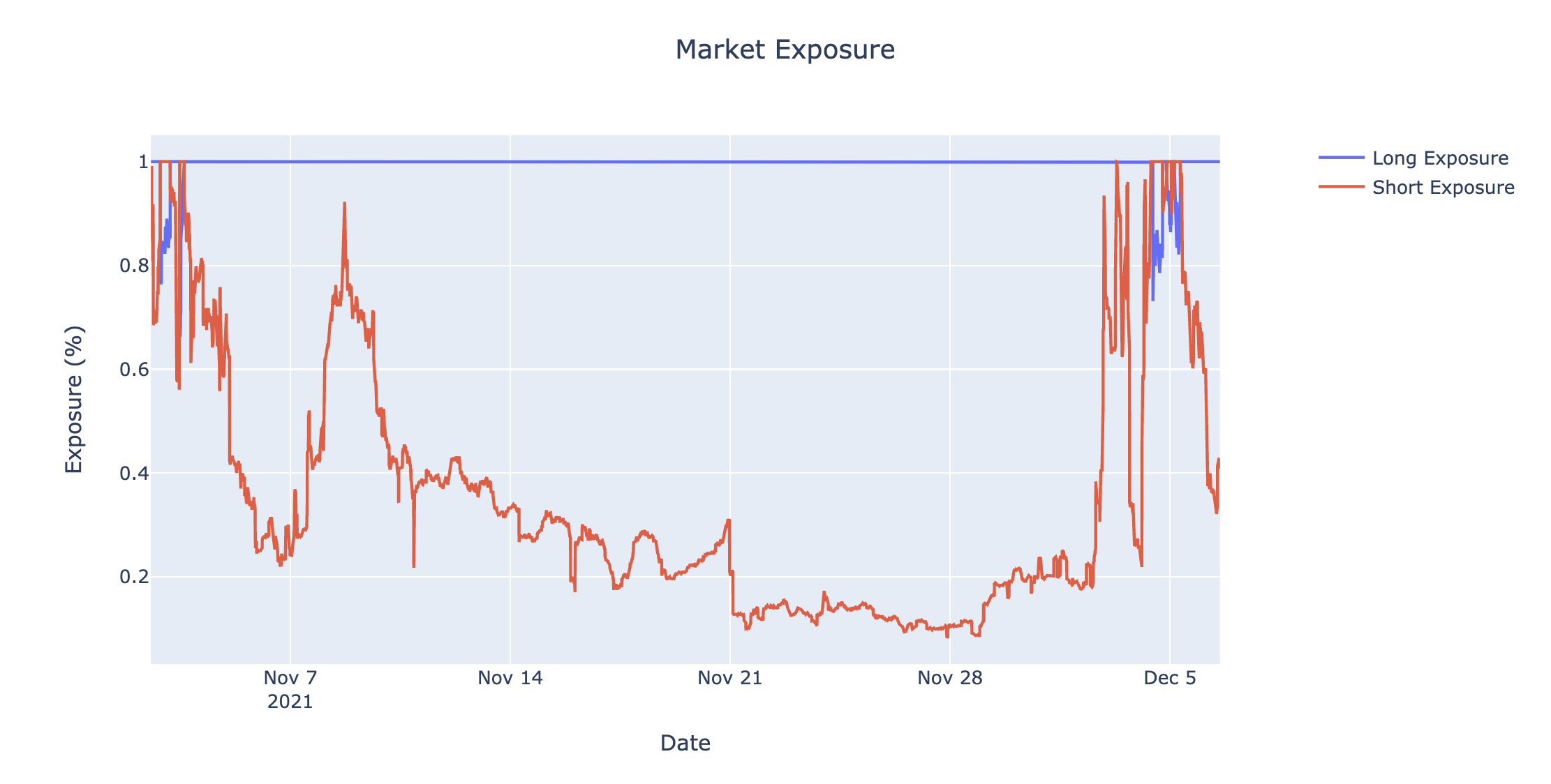
The greater the exposure to leveraged movements, the greater the [absolute] volatility decay. Our floating exposure mechanism means that the overbalanced side of a market will have a smaller degree of volatility decay experienced, as exposure will be less than 100%.

For the 2-OHM market, the exposure on the short side has been gradually decreasing, and therefore the size of absolute volatility decay has been decreasing as well – graph below.

Leverage employed

Currently our first 2 markets (Flipp3ning and 3TH) have 3x leverage, whereas our third market has 2x leverage on OHM. When it comes to leverage, there is a trade-off between capital efficiency and volatility decay.

For a user wanting to gain vanilla $1000 long exposure to OHM, it means that user has to only mint $500 on long 2-OHM (assuming exposure of 100%) to gain this exposure, allowing users to allocate their capital more efficiently.

However, the greater the leverage the greater the potential for volatility decay, and one way to find the correct balance is to observe the historical volatility decay in our markets and see whether they are at acceptable levels.

Absolute difference in price between entry and exit

The greater the difference in underlying price of the asset ‒ from the time a user enters the market to the time that they exit ‒ the greater the [absolute] volatility decay. For example, if a user enters a market when the price of the underlying asset is $100 and then exits when the price is $200, they would experience greater volatility decay than if they exited when the price was $150. The same goes for negative price movements. Note that the volatility decay is not necessarily 0 if the user exited at the same price that they entered.

Magnitude of underlying price movements

Float Capital updates user’s positions when the oracle price feed of the underlying asset gives a new price. The higher the change in the underlying price, the higher the volatility decay will be for any users with active positions at the time of price update. This effect is compounded when there are multiple price updates of high magnitude in the same direction, and is dampened when there are multiple price updates of high magnitude in opposite directions. For example, if there are 2 positive price movements (not necessarily consecutive) of high magnitude then the volatility decay is higher than if there was 1 positive and 1 negative of the same magnitude.

Note that the only time a user’s volatility decay is affected by large single price movements is if they hold a position in the market at the time of the price movement i.e. historical price movements do not affect new investments.

So how high is high? This is something that will be explored in detail in the next blog. But very basically: the relationship between the magnitude of a single price movement and the resulting volatility decay is linear (whose factor/gradient is dependent on the market leverage less 1), and is offset by the volatility decay before the price offset. For [a rough] example, if the current volatility decay for a user in a 2x leveraged market is 01% and the magnitude of the next price update is 10% then the resulting volatility decay is also 10% ; and in a 3x leveraged market it would be 20%). Note that this is a rough example and may not be entirely accurate.

The higher the inherent volatility of the asset, greater the potential volatility decay.

To reduce the volatility of the underlying asset as much as possible, Float uses a deviation threshold of 0.5% and a maximum heartbeat of 5 minutes (actually heartbeat for 3TH market is 27 seconds), asset by our oracle provider, Chainlink.

This means that the price feed will at least update every heartbeat, but also update sooner if the price changes by more than 0.5% from the previous price.

Volatility Decay for short side of 2-OHM market

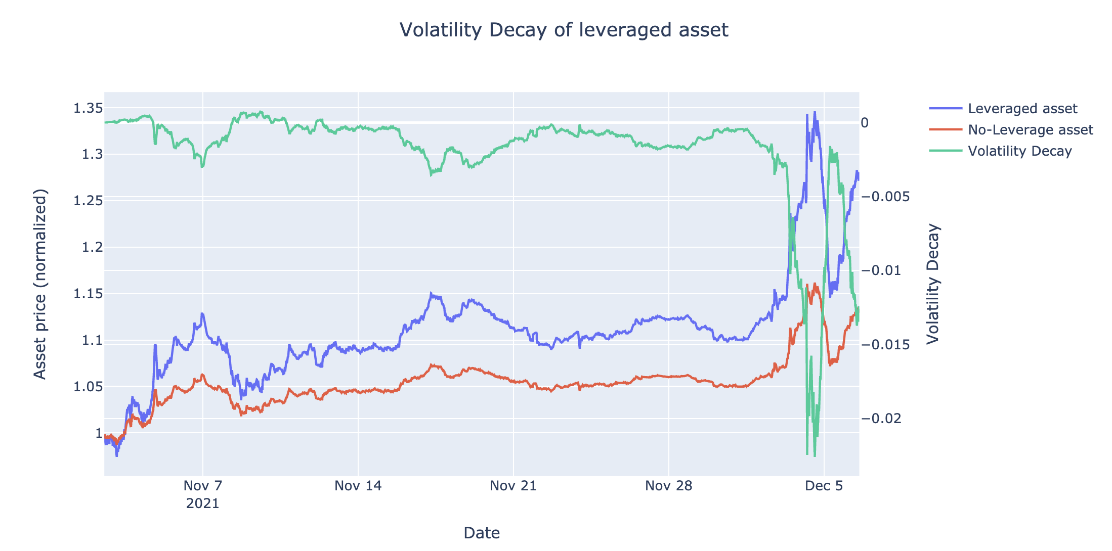
This graph shows the cumulative returns of 2-OHM (in blue) and OHM (in red) for the short side, as well as the volatility decay so far (in green) assuming that someone had entered the market from 2 Nov 2021 when market was created.

We see that volatility decay dropped to -2% in around 5 December 2021, which means that someone holding short 2-OHM would have outperformed someone holding twice the amount in vanilla OHM by 2%.

We have observed volatility decay from the short side above – what does this look like on the long side? A similar calculation can be done for volatility decay on the long side, which does not necessarily produce an equal and opposite value to the short volatility decay.

It is also important to note that because Float Capital is a peer-to-peer market, volatility decay is both positive and negative, meaning generally volatility decay for one side is a gain for the other side.

For example, if the long side has experienced a 0.9% volatility decay over a 7-day period, then that 0.9% is retained by the short side.

In Summary

Volatility decay is something inevitable when it comes to leveraged assets, and the best is to put measures in place to limit its size.

In the article, we explored the mechanisms in place on Float Capital (such as floating exposure and our current practice with Chainlink) which reduce the size of volatility decay as much as possible for users.

One view that could be taken toward volatility decay is that it is the cost of using a capital efficient asset, which is achieved by employing leverage.

The amount of liquidity that did not shift as a result of volatility decay, will remain on the opposite side of the market (i.e. opposite side benefits from volatility decay on one side).

More technical deep dive coming soon for the wrinkle-brained Floatonians.

If you want to learn more about Float Capital, check out our docs, read our whitepaper, or join our Discord.

This piece was written by Woo Sung Dong and Stent (Anon).